")
This is the second chapter of a three-part series on Evolutionary Feature Selection with Big datasets. We will start where we left off, namely with a review of existing metaheuristics with special focus on Genetic Algorithms as they are the base of the CHC algorithm, which we will develop in Part 3 of this series.
Metaheuristics for optimization
There are four main classes of metaheuristics:
1. Local Search metaheuristics: depart from initial solution and explore its neighbourhood, i.e. solutions that differ only in a few components. Some prominent examples are:
(a) Tabu Search, in which complex memory structures are built during the search which forbid already explored solutions
(b) Simulated Annealing, inspired by the metaphor of a crystalline solid cooling down, which continuously decreases its energy but presents some occasional increments. Analogously, the algorithm moves to better neighbour solutions but also permits moving to worse solutions with a small probability that decreases along time.
(c) Variable-Neighbourhood Search (VNS), which starts exploring the nearby neighbourhood but goes on to outside neighbourhoods if it cannot find improvements in the nearby ones.
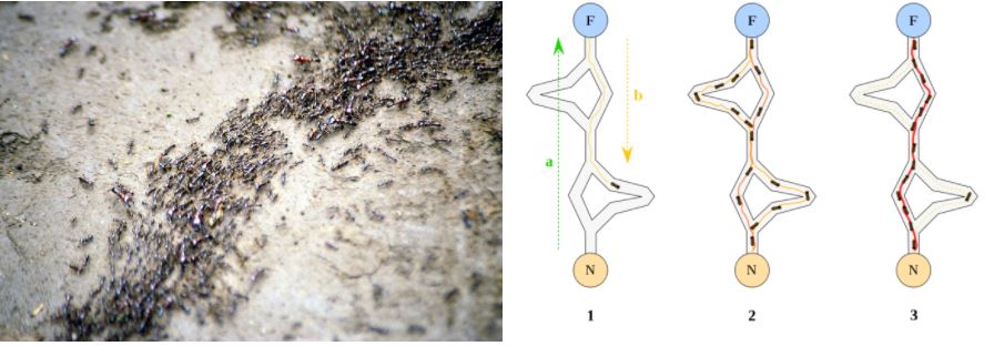
2. Constructive metaheuristics: construct a solution from its parts. Classical examples are GRASP (Greedy Randomized Adaptive Search Procedure) and Ant Colony Optimization (ACO). The latter build solutions according to past pheromone trails (metaphor): pieces of the solution that were part of a good solution in the recent past have higher probability of being chosen when building new solutions. This technique requires reformulating the optimization problem as a path finding problem in a graph, although this can be done surprisingly easier than one might think. The typical problem ACO solves is the TSP (Traveling Salesman Problem), which is already a graph route problem itself.
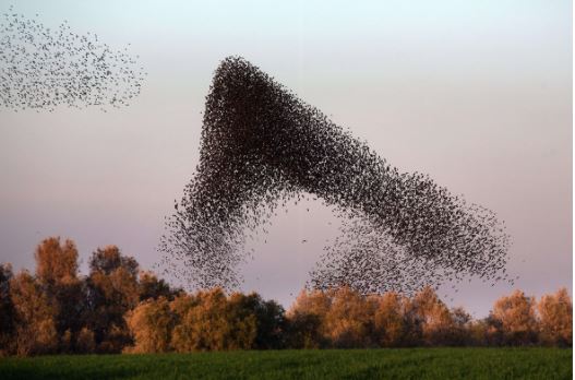
3. Swarm Intelligence metaheuristics: a group of simple, homogeneous agents cooperate to find the best solution, like in Ant Colony Optimization or Bee Colony Optimization. An interesting subclass of metaheuristics are Particle Swarm Optimization (PSO), in which moving particles influence each other as a flock of birds does.
What is interesting about swarm intelligence is the fact that very simple agents (be it a living being or a procedure in a computer program) with no explicit leader can exhibit very complex emergent behaviour through simple communication strategies between them, as demonstrated by the following photographs.
Although ACO and PSO work very well in practice, lots of other (useless) nature-inspired optimization algorithms -beyond swarm intelligence- have been published in the last decade, relying on metaphors such as bacterial foraging, river formation, biogeography, musicians playing together (Harmony Search), electromagnetism, gravity, colonization by an empire, mine blasts, league championships or clouds. The animal behaviour in particular has been widely mirrored in algorithms: ants, bees, bats, wolves, cats, fireflies, eagles, vultures, dolphins, frogs, salmon, termites, flies…
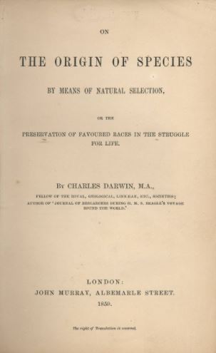
4. Population-based metaheuristics: group of solutions (called chromosomes) evolve together as in natural evolution (as proposed by Charles Darwin’s The origin of species in 1859). There are four sub-classes of strategies here:
4.1. Genetic Algorithms (GA), first developed in 1975 in Michigan University: chromosomes (solutions) evolve through crossover and mutation.
4.2. Genetic Programming, first developed in 1989 at Stanford University: the solutions are expression trees which evolve and cross. For instance, symbolic regression in which there is no predefined shape for the regression curve: the shape is also part of the search.
4.3 & 4.4: Evolution Strategies (ES) developed in 1964 in Berlin (CMA-ES is a very well-known algorithm for continuous optimization that falls in this class and has very good performance) and Evolutionary Programming, developed in 1966 in Florida: in both approaches, populations evolve without crossover operation.
Genetic Algorithms
They are probably the most extended evolutionary approach due to their ease of implementation. The workflow of a Generational Genetic Algorithm (GGA) is the following:
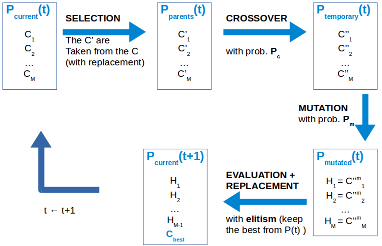
At the initial generation, a set of M (typically between 50 and 200) candidate solutions (in our case, M binary vectors of length N) are generated randomly (the generation mechanism may vary). From them, and using some of the strategies we will comment later, M solutions are selected (with replacement, hence some may possibly appear more than once) to form the parents population. They are mated in random pairs and each pair will cross with a certain probability Pc (which is normally quite high, between 0.7 and 0.9) to generate two offspring (when the parents do not cross, the offspring is assumed to be the parents themselves). Then, each of the the M resulting offspring may suffer a spontaneous mutation with a probability Pm (which is normally low, between 0.1 and 0.3). The resulting individuals are then evaluated according to certain fitness function, which in our Feature Selection problem is the performance of a k-NN classifier on the input data with the selected feature subset, as will be explained in the next section. Finally, the new population replaces the old one completely (this is the case for a Generational GA) and the loop repeats again. The stopping criterion consists in calling the fitness function a maximum number of times.
In a different variant, called Stationary GA, only two individuals are selected as parents, crossed and mutated, so the offspring only replaces two individuals -either at random or the two worst solutions- from the old population. Most often, the algorithm incorporates elitism, meaning that the best solution from the old population is always kept and replaces the worst solution from the newly generated population. We will later define some crossover and mutation operators commonly used in GAs. As can be seen, a GA depends on several parameters, such as the number of individuals of the population, M, the crossover and mutation probabilities, Pc and Pm, and the maximum number of fitness evaluations allowed.
Components needed to apply a GA to a specific problem:
- Design a representation (e.g.: binary vector), and a correspondence between genotype and phenotype (what the binary vector means: 1 means to select that feature, 0 means to drop that feature).
- Decide how to initialize the population at generation 0 (usually random).
- Design a way to assess an individual (fitness function).
- Design suitable crossover and mutation operators for the problem at hand (offspring feasibility).
- Design a parent selection mechanism.
- Design a replacement mechanism (generational, steady-state).
- Decide the stopping criterion (number of evaluations of the fitness function).
In the next (and last) chapter, we will briefly comment on some options available for the aspects above, and we will explain in detail the characteristics of CHC and how it can be parallelized.


