")
This is the last chapter of the three-part series on Evolutionary Feature Selection with Big datasets. We will continue where we left off, addressing some fundamental design aspects of a Genetic Algorithm (GA) and commonly chosen options, to then move on to the CHC algorithm and a distributed approach for Feature Selection.
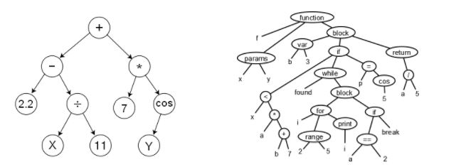
The genotype-phenotype correspondence: a genotype is the computational representation, while a phenotype is the concept represented. For instance, a binary vector may represent which features are selected or dropped in a Feature Selection problem, or which instances are selected or not in an Instance Selection problem, or a sequence of behaviours that have arisen or not. A sequence of integers could represent a solution to a real optimization problem but also a permutation, meaning the order in which certain tasks must be accomplished. In genetic programming, individuals are encoded by trees, which represent phenotypes such as an algebraic expression or even a whole computer program (see below).
Parent selection mechanisms: The best individuals should have a higher probability of being selected as parents, but not-so-good individuals should also have a chance. The parent selection mechanism heavily affects the selective pressure, which has an impact on the speed of convergence. Some choices are:
- k-ary tournament selection: select k individuals at random and pick the one with the best fitness value. Higher k entails higher selective pressure and thus, faster convergence, but we might end up in a not very good local optimum.
- Randomized, proportional to ranking: sort the individuals by their fitness, and select a parent with a probability linearly proportional to the ranking (ignoring the exact fitness).
- Randomized, proportional to fitness (roulette): the same as before, but select with probability proportional to the exact fitness value (this is a classic choice).
- Negative assortative mating (NAM): pick one parent randomly, P1. Then select k candidates and pick the one which is most different from P1. It is aimed at introducing diversity.
Crossover operators: the offspring should inherit some characteristics of both parents; otherwise it is not a crossover operator but a mutation. It is usually applied with high probability. It is important to check the feasibility of the offspring. Some common options are:
- k-point crossover. The exact steps of the operator depend on the genotype-phenotype correspondence to avoid generating unfeasible offspring.
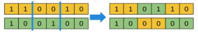
For a binary vector genotype: example of a 2-point crossover
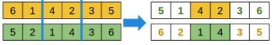
For a permutation genotype: take a fragment from one parent, and sort the remaining elements as in the other parent.
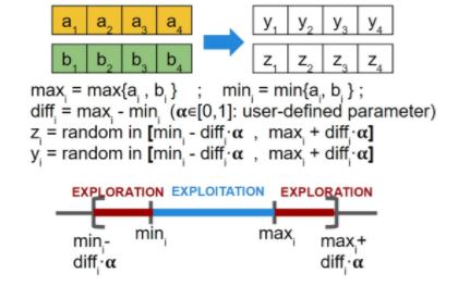
- BLX-? (where ? is a configurable parameter in [0, 1]): suited for real parameter vector genotypes: for each gene, compute the min and max of both parents, and choose a random value that can be either in between, or be a percentage smaller than the minimum or greater than the maximum.
Mutation operators: should be designed so that any region of the solution space can be reached. Again, the mutated individuals must still be feasible solutions. It is usually applied with low probability. The following are some common mutation operators:
- Binary vector: each gene has probability Pm of being flipped:
![]()
- Permutation: if the individual is mutated (which happens with probability Pm), then switch two positions at random.
![]()
- Real vector: each gene has probability Pm of being perturbed as follows:
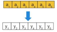
If ai is selected for mutation (with probability Pm), then yi = ai + N(0, ?i ) where ?i controls the intensity of the perturbation, which may vary along the algorithm to allow for strong perturbations at the beginning (more exploration) but soft at the end (to favour exploitation). If ai is not selected, then yi = ai.
The CHC algorithm for Feature Selection
It was introduced in a paper of 1990 presented at the First Workshop on Foundations of Genetic Algorithms (see [1]). It is a binary-coding genetic algorithm with high selective pressure and elitism selection strategy, with additional components that introduce diversity. The inventor of CHC, Larry Eshelman, defines it as a Genetic Algorithm with some key modifications.
- Half Uniform Crossover (HUX): randomly select half of the genes that are different between the parents, and exchange them. This maximizes the Hamming distance between the offspring and their parents (see the paper for the theoretical motivation).
- Elitist population replacement: join the current and the offspring populations together, and then select the M best individuals to form the new population.
- Incest prevention: M/2 pairs are formed with the elements of the population. In each pair, if the individuals should cross according to the crossover probability, they are not allowed to finally mate if their Hamming distance exceeds a threshold ? (usually initialized to ? = ?/2, where ? is the chromosome length), meaning they are too similar. The threshold is decremented by 1 when no offspring is obtained in one generation, which indicates that the algorithm is converging.
- Restarting process: when ? = 0 (several generations without any new offspring), the population is considered to be stagnated and a new population is generated: the best individual is kept, and the rest are strongly mutated (using the existing individuals as templates for generating new individuals).
The fitness function for the FS problem: up to now, we have said nothing on the fitness function needed to evaluate individuals (candidate solutions, i.e. feature subsets) when applying CHC (or any other GA) to the FS problem. If the reduced dataset is to be used in a classification task, it would be ideal to use the same classifier as the fitness function to guide the search, but a wrapper method is computationally expensive and the fitness function is called so many times. Hence, it is better to pick some fast classifier. Actually it is enough to distinguish which of two individuals is better, and be right, no matter the exact fitness value.
A proposal is to use the performance of a k-NN classifier on the dataset with the selected features and Leave-One-Out (LVO) to classify each example. In the paper [2], the authors took k = 1 (nearest neighbour classifier). Furthermore, since the datasets given as input may be imbalanced, the authors advise to use the Area Under the ROC curve (AUC) instead of accuracy. AUC is defined as AUC = (True Positive Rate + True Negative Rate) / 2. Finally, because the aim is to select features, the fitness function should be a weighted sum of the AUC and the feature reduction rate:
Fitness = 0.5 x AUC + 0.5 x Reduction rate = 0.5 x AUC + 0.5 x (1 – (#Fselected/#Ftotal))
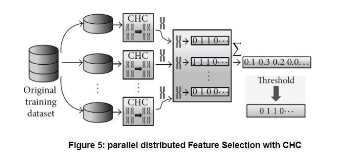
Parallel Feature Selection with CHC for Big datasets: the original proposal [1] implemented CHC with Hadoop MapReduce in Java, though we are now re-implementing it with Apache Spark. The dataset is divided into chunks (partitions), which fit into the workers’ memories. A sequential (non parallel) CHC is applied locally to each chunk, using 1-NN with LVO as fitness function, as explained above. The local results are binary vectors (one per partition), which are aggregated by computing the average per gene. Finally, the vector of averages is binarized again: the elements above a certain user-defined threshold are considered as selected features, i.e. the threshold regulates the severity of feature selection. The figure below shows the process. The local and aggregate method works quite well with other algorithms too; research is being done on the Instance Selection problem following the same approach.
What follows is a brief summary of the results presented in [2].
A simple time complexity analysis: as explained in [2], CHC is in O(n2 Dp) where n is the number of examples, D is the number of features, and p is the maximum number of fitness evaluations allowed. When we divide the data into m chunks, the complexity of each local CHC on a chunk is in O((n2/m2)Dp). If we run them sequentially (one after another), the total is m times larger, i.e. it is in O(m(n2/m2)Dp) = O((n2/m)Dp). This is already faster than running a global CHC on the complete dataset. If we have nc cores available (instead of just one) to run several local CHCs in parallel, the total time is in O(⌈m/nc⌉(n2/m2)Dp).
The authors of [2] used a 240-core cluster. The datasets evaluated were the following:
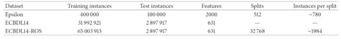
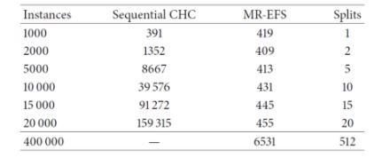
It can be seen that the sequential CHC takes a long time to run, and needed too long for the case of the full 400.000-instance dataset. Contrary to this, the distributed approach scales quite well, although takes 6531 seconds (almost two hours) to complete with the full dataset. Since 400.000 instances is not a really large dataset, the experiments confirm that, while able to scale up, even the distributed approach is computationally heavy. Next, we examine the effects of feature selection on the performance of three different classifiers, namely a logistic regression, a Naive-Bayes and an SVM (tested with two different regularization parameters, 0.0 and 0.5), trained on the reduced datasets resulting from the FS process.
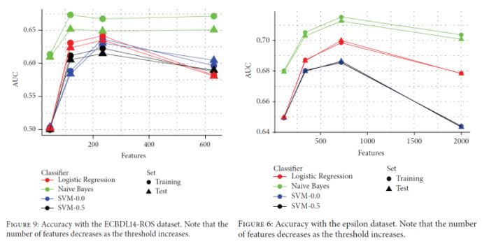
It can be seen in both cases that having less features may boost the classification performance. In the ECBDL14-ROS dataset (a balanced version of ECBDL14 after random oversampling), having around 240 features leads to the best results except for Naive Bayes (and even in this case, the gain in performance with the full 600 features is very small). In the Epsilon dataset, the AUC reaches the maximum when having around 750 features instead of the total 2000 features.
Conclusions
In this three-part series we have seen how Feature Selection can be approached as a combinatorial optimization problem in the feature subset space, and solved by an intelligent search performed by a metaheuristic. After presenting a taxonomy of metaheuristics, we have focused on Genetic Algorithms and some design choices when applying a GA to a problem. Finally, we have explained the characteristics of the CHC algorithm in the general context of a GA, and how it can be used in a distributed manner to perform feature selection on big datasets that are distributed across a cluster of computers. The idea of running CHC locally (and if possible, simultaneously taking advantage of several cores in a cluster) on separate chunks of the original input data (each chunk includes all the features but only a subset of the examples) gives good results and improves the performance of subsequent classifiers built on the reduced feature set. As soon as we finish our Spark implementation we will report the results, which we expect to be at least as promising as those in [2].
References
[1] The CHC Adaptive Search Algorithm: How to Have Safe Search When Engaging in Nontraditional Genetic Recombination. In: G. J. E. Rawlins (Ed.): Foundations of Genetic Algorithms, vol I, pp. 265 – 283. California, Morgan Kauffman Publishers Inc. (1991)
[2] Peralta, D., Del Río, S., Ramírez-Gallego, S., Triguero, I., Benítez, J.M., and Herrera, F. Evolutionary Feature Selection for Big Data Classification: A MapReduce Approach. Mathematical Problems in Engineering, vol. 2015, Article ID 246139 (2015)
[3] Slides of the course on “Bioinformatics” by F. Herrera (in Spanish). University of Granada, Spain http://sci2s.ugr.es/graduateCourses/bioinformatica (chapter 6)
[4] Goldberg, D. Genetic Algorithms in Search, Optimization & Machine Learning. Addison-Wesley, 1989.


